Methodological Review of GWR and MGWR 
Notebook Outline:
Local Regression Models
Geographically Weighted Regression (GWR)
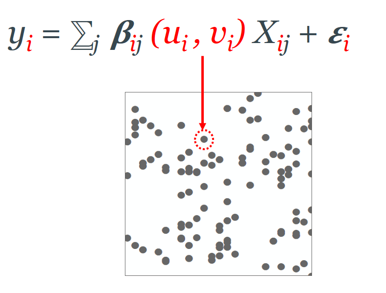
Since the global models provide an average coefficient estimate for each predictor variable across the study area, they inherently assume the relationships tp be constant across space. That is however, not always true. GWR relaxes this assumption and provides a unique coefficient estimate for each location and for each covariate. The GWR model is essentially an ensemble of OLS regressions calibrated at each individual location of the study area which is reflected by the (ui,vi) in the equation here.
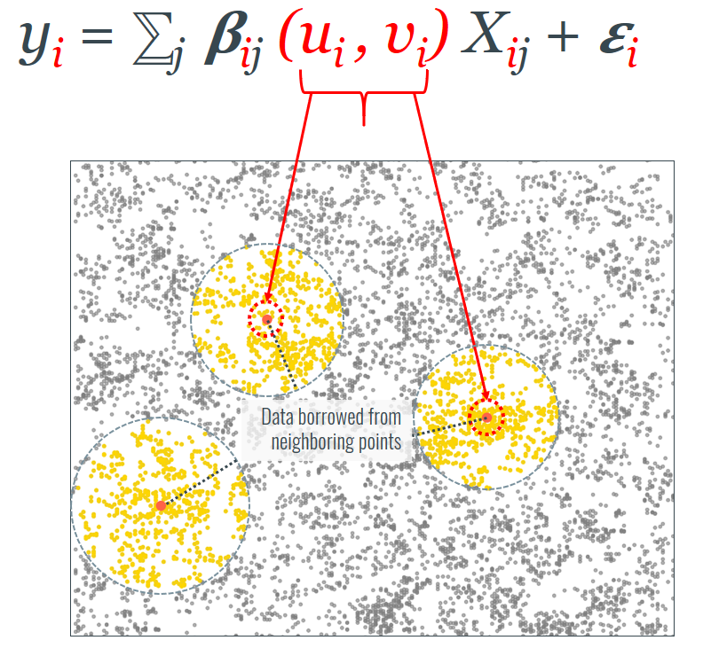
To calibrate a regression model at each location we would technicaly require multiple unique data points at the same location. Since that kind of data is extemely hard to find, GWR gets around the problem by borrowing data from geographically neighboring locations. This is in accordance with Tobler's Law of spatial dependence. The number of neighboring data values used to calibrate a model is obtained using an optimization criterion such as Akaike Information Criterion (AIC) or cross-validation and the parameter thus obtained is called the bandwidth. The bandwidth is interpreted as an indicator of scale at which the spatial processes have the most to contribute to the formation of the spatial pattern being examined.
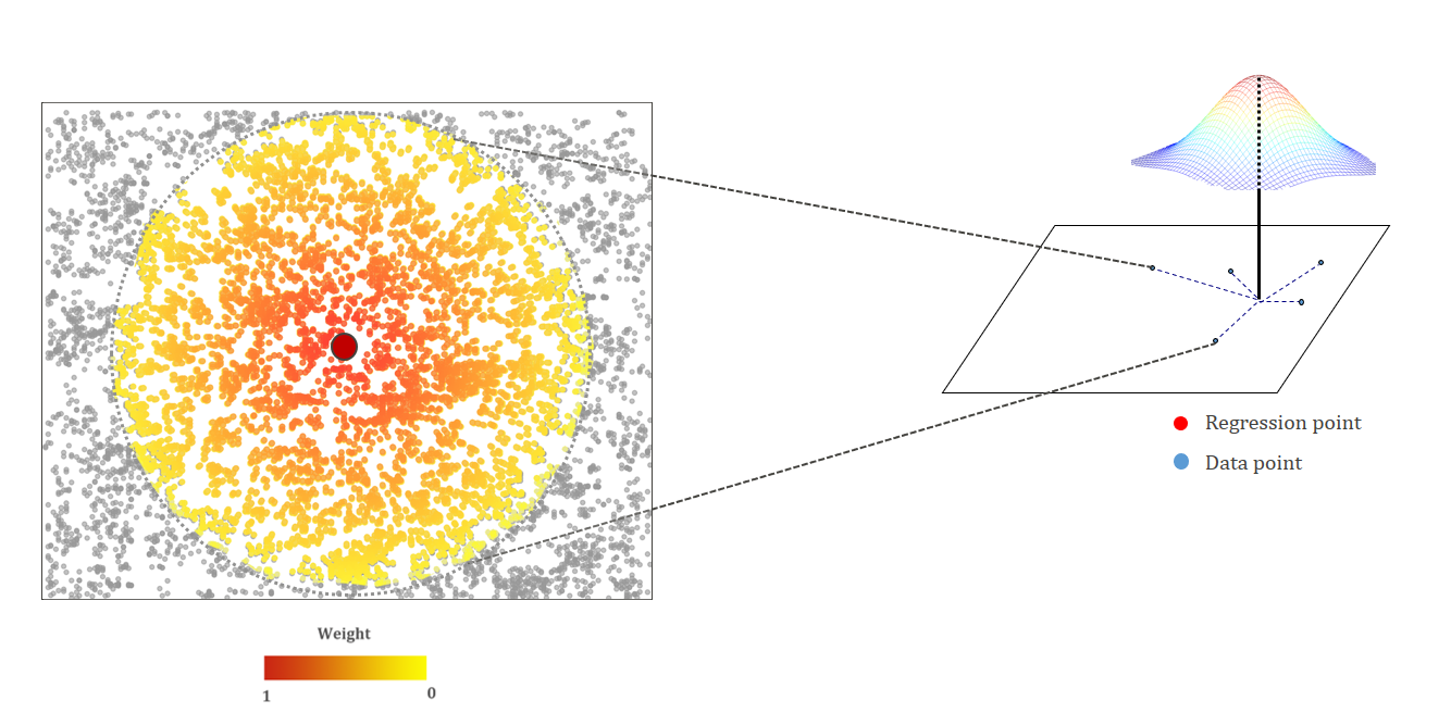
In effect, the bandwidth parameter in Geographicallly Weighted Regression, refers to the width of the kernel within which observations are weighted and used in the calibration of the local, site-specific model. A large bandwidth hence, would indicate that observations farther away from the point of calibration are included in the loca model than in the one with a smaller bandiwdth. The bandwidth can thus be interpreted as a measure of the extent of overall spatial heterogeneity in relationships. Large bandwidths in a model would indicate broad spatial variation in relationships and as the size of the bandwidths decreases, more detailed patterns in variation of spatial relationships becomes visible.
A weighting kernel in GWR can be chosen between an adaptive bisquare function and a fixed Gaussian function. For the adaptive bisquare kernel, the weights are assigned to the same number of points across space (nearest neighbors) and the bisquare function is used as a diminishing function. The fixed kernel, on the other hand, is more appropriate in situations where the data are more evenly spread and a fixed distance for defining a subset of local data used for calibration can be justified.
Multiscale Geographically Weighted Regression
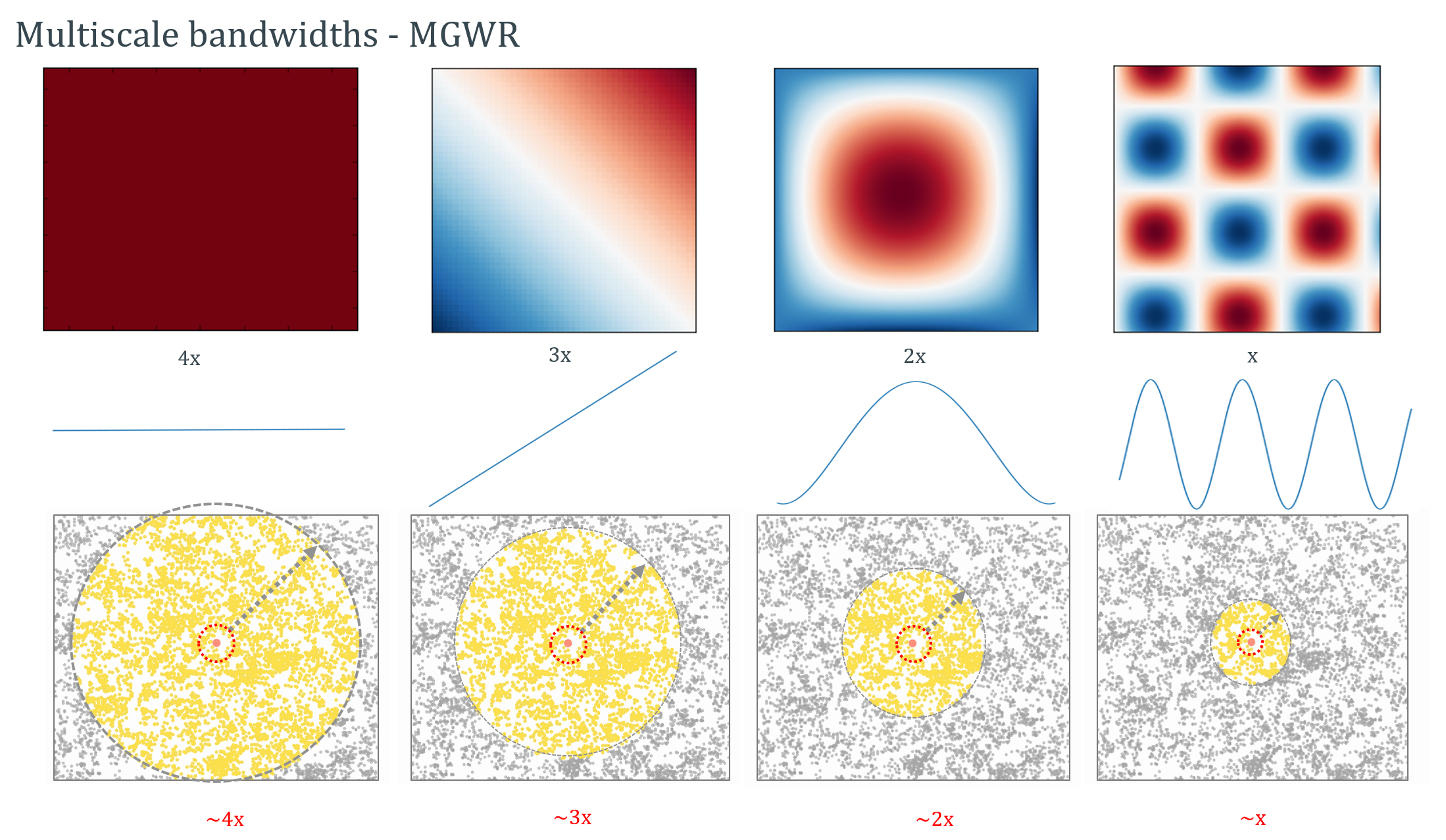
Since different processes affect the spatial pattern we observe at different scales (as we discussed previously in the human migration example), a multiscale extension to GWR was recently developed. This extension relaxes the assumtion that all processes operate at a single scale and allows the estimation of unique scales of spatial processes in a model.
In the simulated example below, for example, an MGWR model will potentially be able to estimate an appropriate scale for each process depending on the amount of spatial heterogeneity in each process. MGWR model in effect, produces a bandwidth parameter for each spatial process being modeled (i.e. one bandwidth paremeter for each of the betas associated with the independent variables).